How to Calculate Compound Investment Returns and Compare Them with Charts

Introduction

If you invest a fixed amount every month or year, how much could the portfolio be worth in the future? Adding the initial investment to total contributions gives the principal, but the future value also depends on how long each contribution remains invested.

This article starts with the simulation and charts. The geometric-series derivation is kept as an optional supplement at the end.

The 2%, 4%, and 6% rates below are constant-return assumptions used for illustration. Actual investments fluctuate, and future results are not guaranteed.

1. Simulation assumptions

Item	Assumption
Initial investment `P₀`	JPY 1,000,000
Annual contribution `C`	JPY 120,000 at each year-end
Investment period `n`	30 years
Assumed annual return `r`	0%, 2%, 4%, and 6%
Excluded	Fees, taxes, and inflation

For contributions made at each year-end, the future value after n years is:

S_n = P₀(1 + r)ⁿ + C (1 + r)ⁿ − 1r

When the assumed return is 0%, use S_n = P₀ + nC. The derivation appears at the end.

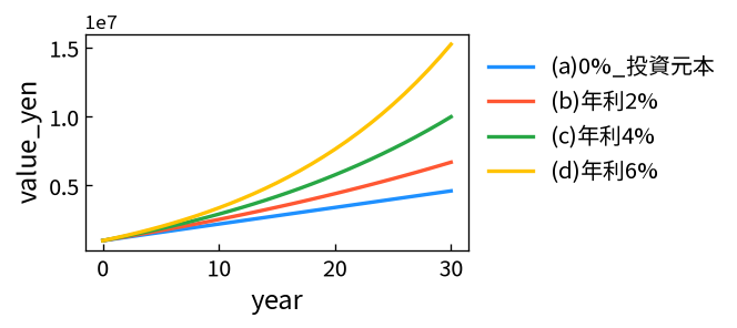
2. Comparing 0%, 2%, 4%, and 6% assumed returns

Portfolio values at assumed annual returns of 0, 2, 4, and 6 percent — Figure 1: Portfolio value by assumed annual return, created with Sakura Chart. The 0% line is the principal reference.

Years	0% principal	2%	4%	6%
5	JPY 1.60M	JPY 1.73M+JPY 0.13M vs principal	JPY 1.87M+JPY 0.27M vs principal	JPY 2.01M+JPY 0.41M vs principal
10	JPY 2.20M	JPY 2.53M+JPY 0.33M vs principal	JPY 2.92M+JPY 0.72M vs principal	JPY 3.37M+JPY 1.17M vs principal
15	JPY 2.80M	JPY 3.42M+JPY 0.62M vs principal	JPY 4.20M+JPY 1.40M vs principal	JPY 5.19M+JPY 2.39M vs principal
20	JPY 3.40M	JPY 4.40M+JPY 1.00M vs principal	JPY 5.76M+JPY 2.36M vs principal	JPY 7.62M+JPY 4.22M vs principal
30	JPY 4.60M	JPY 6.68M+JPY 2.08M vs principal	JPY 9.97M+JPY 5.37M vs principal	JPY 15.23M+JPY 10.63M vs principal

Total principal after 30 years is JPY 4.60 million. The simulated differences from principal are JPY 2.08 million at 2%, JPY 5.37 million at 4%, and JPY 10.63 million at 6%. The green values in the table show the difference from principal at each point. The gap becomes wider over longer periods because growth compounds.

3. Create charts from two ready-to-use datasets

Use the standard chart builder for the four-rate comparison, or the combination-chart builder to show principal, portfolio value, and gain rate together. Each button sends the sample data directly to the appropriate tool.

3-1. Standard chart data: long format by assumed return

Select year for X, value_yen for Y, and LEVEL for the legend, then choose a line chart.

year,value_yen,LEVEL
0,1000000,(a)0%_principal
1,1120000,(a)0%_principal
…
0,1000000,(c)4%
1,1160000,(c)4%

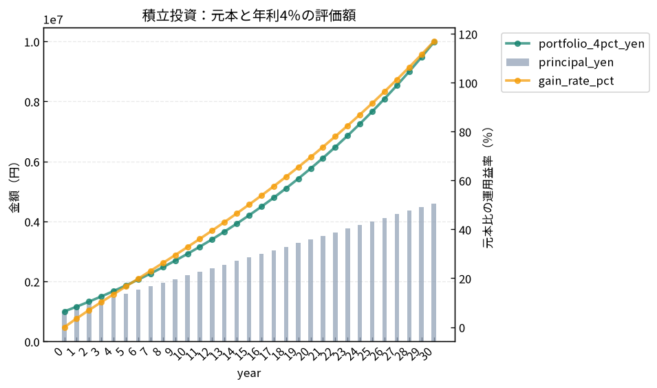
3-2. Combination chart data: principal, portfolio value, and gain rate

Principal is shown as bars on the left axis, the 4% portfolio value as a line on the left axis, and gain rate as a line on the right axis.

year,principal_yen,portfolio_4pct_yen,gain_rate_pct
0,1000000,1000000,0
1,1120000,1160000,3.57
2,1240000,1326400,6.97
…

A combination chart showing principal, portfolio value at 4 percent, and gain rate — Figure 2: A Sakura Chart combination chart showing principal, portfolio value at 4%, and gain rate.

4. Adapting the calculation to monthly contributions

If R is an effective annual return, the equivalent monthly rate is i = (1 + R)^1/12 − 1. Use the same future-value formula with monthly contribution c and N = 12n months. Products and calculators may use different timing and rate-conversion conventions.

5. Important limitations

Actual returns vary and may be negative.
Beginning-of-period contributions remain invested longer than end-of-period contributions.
Fees, taxes, and inflation affect real outcomes.
A simulation is not a forecast or guarantee.

Japan's Financial Services Agency states in its investment simulator that simulations do not predict or guarantee future results. GPIF also explains that future returns are not fixed in What is investment risk?

6. Summary

Each contribution grows for a different length of time.
Differences between assumed returns widen over long periods through compounding.
Principal provides a useful reference for separating contributions from simulated gains.
Use long-format data for the standard chart and wide-format data for a combination chart.

7. Supplement: deriving the recurring-investment formula

This optional section explains the geometric-series derivation.

Open the derivation

S₁ = P₀(1 + r) + C

S₂ = P₀(1 + r)² + C(1 + r) + C

After n years, the contribution terms form a geometric series:

C{1 + (1 + r) + … + (1 + r)^n-1}

Applying the geometric-series sum and adding growth on the initial investment gives:

S_n = P₀(1 + r)ⁿ + C(1 + r)ⁿ − 1r

For beginning-of-period contributions, multiply the contribution term by (1 + r).